The Shape of Uncertainty: How Covariance Explains Noise in 3D Space

In the early 19th century, deep in the observatories of Göttingen, Carl Friedrich Gauss was quietly refining a theory that would reshape how we think about uncertainty. It wasn’t the drama of Newtonian gravity or the fireworks of electricity and magnetism—this was something subtler. He was studying measurement error.

Gauss proposed that error followed a bell curve—not by divine decree but as a mathematical consequence of random disturbances adding together. The famous Gaussian distribution was born. But Gauss gave us something even more powerful, almost unnoticed at the time: the concept of covariance.

Today, covariance—especially covariance matrices—has become the language of how we understand noise in three-dimensional space. From spacecraft navigation to earthquake sensing, from financial markets to machine learning, covariance tells us not just how uncertain we are, but in what direction.

Let’s take a walk through this world of noisy vectors.

The Intuition: From Points to Clouds

Imagine you’re standing in the middle of a foggy field, trying to locate the position of a lost drone. You hear a faint beep—it’s trying to tell you its GPS coordinates. But the reading is noisy.

Now suppose you receive not just one reading, but hundreds. Plot them all in 3D space, and you get a cloud of points.

If the noise was identical in all directions (i.e., isotropic), you’d see a sphere. But real-world noise rarely behaves so politely.

Instead, you might see a cloud stretched along a diagonal, like a cigar pointing northeast. That’s covariance in action. The cloud has a shape because the noise has directional structure—some directions are more uncertain than others.

The Mathematician Behind the Shape: Andrey Kolmogorov

Fast-forward to the 1930s. The Russian mathematician Andrey Kolmogorov formalized the field of probability theory. He gave us the modern axioms, but more importantly, he made it rigorous to talk about random vectors. In 3D, a random vector might represent the noisy measurement of a position:

 x = [x₁, x₂, x₃]ᵗ

The covariance matrix of x tells you how much each coordinate varies and how much they vary together:

 Σ = E[(x - μ)(x - μ)ᵗ]

Where μ is the mean of the vector.

This matrix is symmetric and positive semi-definite. It holds six unique numbers in 3D: three variances along the diagonal, and three covariances off the diagonal.

This is where things get beautiful.

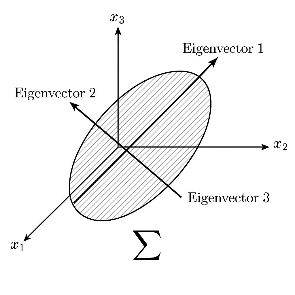
The Ellipsoid of Confidence

Enter Jacques Hadamard, a French mathematician who first formalized the geometric idea of the confidence ellipsoid.

When you plot the covariance matrix as a 3D ellipsoid, you are visualizing the uncertainty. The directions of the ellipsoid’s axes are the eigenvectors of the matrix. Their lengths are proportional to the square roots of the eigenvalues.

• A tall ellipsoid means more uncertainty in that direction.

• A flat ellipsoid means more confidence.

• A tilted ellipsoid means the noise is correlated—errors in x and y move together.

In practice, this tells you how reliable your sensors are, which direction to trust, and how to filter out noise.

The Kalman Whisperer: Rudolph E. Kalman

In the 1960s, an engineer named Rudolph Kalman took these ideas and turned them into the Kalman filter—a recursive way to estimate position, velocity, and more from noisy measurements. NASA used it to guide Apollo missions.

At every step, the Kalman filter maintains a state estimate and an uncertainty ellipsoid, encoded by the covariance matrix:

Predicted Covariance: Pₜ|ₜ₋₁ = A · Pₜ₋₁|ₜ₋₁ · Aᵀ + Q

Here, Q represents the noise in the system itself—modeled as a 3D disturbance.

Think of a robot navigating a factory floor. Its sensors have noise. The floor has bumps. The air has turbulence. All these are encoded in Q.

The robot keeps track of how uncertain it is—not just in where it is, but in which directions it's more likely to be wrong.

Earthquakes and Accelerometers

Let’s take a real-world example.

A smartphone sits quietly on a desk. Inside, a tiny MEMS accelerometer samples vibrations in three axes. Normally, it just logs minor tremors. But during an earthquake, the readings spike.

Engineers use the covariance matrix of the 3D accelerometer data to identify the mode of the tremor—is the energy propagating vertically or horizontally? That tells geophysicists how deep the earthquake was.

The principal direction of the covariance matrix aligns with the fault’s movement. The Earth shakes, and covariance whispers its secrets.

Robotics: Covariance as a Guide Dog

In modern robotics, a drone navigating through a warehouse uses LiDAR and inertial sensors. The 3D position estimate is fused using Kalman filters or particle filters. But the covariance matrix does more than just track uncertainty—it guides behavior.

If the ellipsoid grows too large in a certain direction, the drone knows it's drifting off-course. Some planners use the Mahalanobis distance, which scales Euclidean distance by the covariance, to detect outliers and replan.

Covariance becomes a compass—not just to where you are, but to how confidently you know it.

The Takeaway

Covariance in 3D space is more than a math object. It is:

• The shape of your uncertainty

• The fingerprint of your noise

• The bridge between random motion and informed navigation

From Gauss’s early musings on error to Kalman’s filters and the autonomous systems of today, the story of covariance is the story of how we make sense of a world that refuses to be still.

Whether you are a physicist, a financial quant, or an engineer trying to land a drone, you are living inside an ellipsoid—navigating the fog with a compass made of math.

📚 References & Further Reading

• Gauss and the Method of Least Squares

• The Geometry of the Covariance Matrix

• The Kalman Filter Explained Simply

• Covariance Ellipsoids in Robotics

• Kalman's 1960 Paper on Linear Filtering